Closing the Loop: Building Shapes with a Planar Graph
There’s some fun computational geometry in my latest artwork, and in this article I’ll walk through how I take a scramble of disconnected paths and turn them into closed shapes, using half-edges and a planar graph.

Work in progress output

Work in progress output
Work in progress output
Agent paths
These images begin with a set of “agents” that draw paths. You can think of an agent as a dot that does things (it has “behaviours”).
These agents:
move around the canvas, leaving a trail behind
check whether they’ve run into any existing trails (their own or another agent’s)
when they first run into a trail, they go back to the beginning of their journey and move in the opposite direction.
when the second end hits something, the path is complete and a new agent is generated somewhere else.
Here’s an example with just one agent at a time.
The smooth motion of the agents is controlled using Perlin noise, which is essentially a grid of random numbers. To figure out their next move, each agent looks up the number at their current position and uses it to decide which direction to go in next. For example, if the number is 0 they move at an angle of 0°, if the number is 0.25 they move at 90°, 0.5 at 180°, etc.
If the values in the field were completely random, the agents would jitter back and forth, constantly changing direction wildly. With Perlin noise, numbers that are close to each other in the grid are similar, so the direction only changes a little bit every step, creating a smooth wandering line.
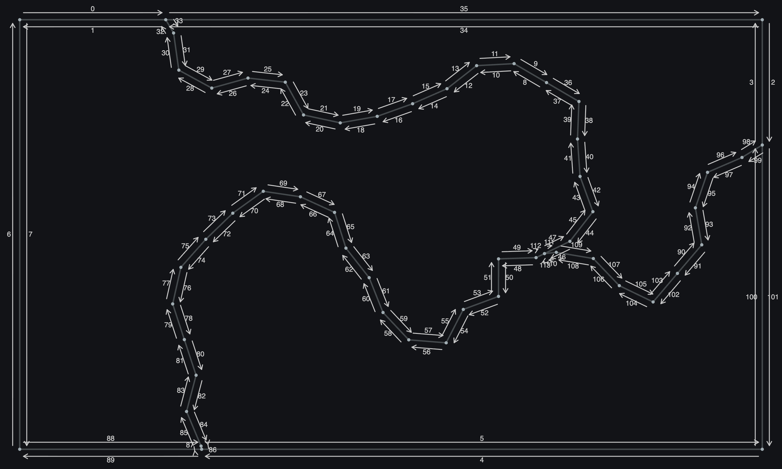
In this animation I’ve drawn a grid of arrows to depict the noise field and you can see the agent following their directions. (As an agent does the second half of its path, it goes backwards along the arrows).
After the agents have been drawing paths for a while, the canvas looks something this.

Agent paths
Right now, what we have is a collection of disconnected paths, one drawn by each agent. They are touching but as far as the computer is concerned, they aren’t connected and these aren’t closed shapes. That means we need to do some work to be able to fill them with colour.
There are lots of approaches for this. Some involve drawing the paths out and then looking at the colours of the individual pixels to know if we’re looking at a path or an empty space. You would pick a starting pixel, change it to a fill colour and then move in lines or spreading outwards until you hit pixels that are already filled with the path colour. I had started implementing that a while ago and had a bug that created these super glitchy images, which I love, even though they weren’t what I had planned.

Glitchy shape filler

Glitchy shape filler
For this new project, I wanted to try joining the disconnected edges into fully closed shapes. Luckily there is an established method for this, a planar graph, so I just had to figure it out.
Vibe coding? More like vibe front-loading
Full disclosure, I had no idea how to do this when I started. I used chatGPT to help me with a first pass at the algorithm and then went through and rewrote all the code so I could understand it and incorporate it into my agents code efficiently.
The AI implementation was re-doing a lot of work that had already been done at the agent stage, like finding the intersections. Fun fact: as I recoded it, I was able to bring it down from 444 lines to around 120, before any real attempts at minifying.
While the Agents Walk
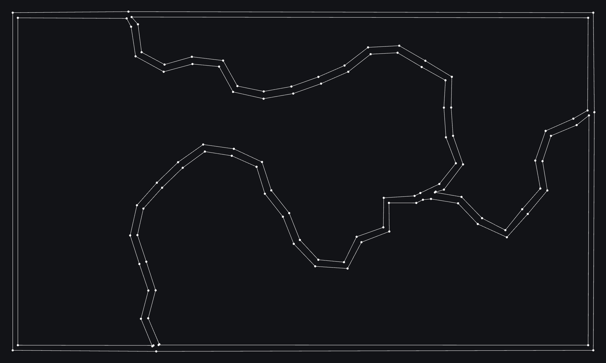
Let’s take a look at a simplified version with just a couple of paths and a bigger distance between the points, so we can see what’s going on.
There is a path that goes around the edge of the canvas, enclosing everything. Usually this is right along the edge but I’ve pulled it in a little so it’s visible.
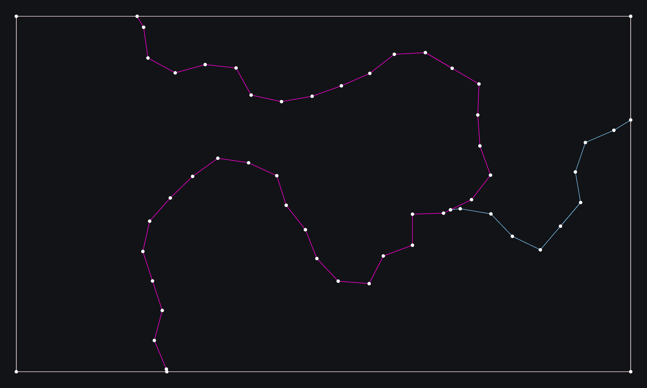
Simple version with two wandering paths plus an outer path
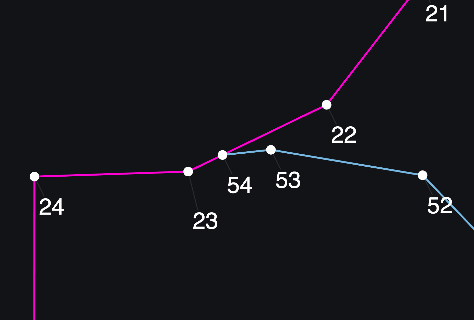
Let’s zoom in on what’s happening where the two wandering paths intersect.
In the images below, we can see that the pink path was created first because the ID numbers of the points are lower. When the blue path came along, it tried to go from point 53 to the location shown with the grey dashed line (first image), which would have been point 54. However, that collides with the existing pink path.
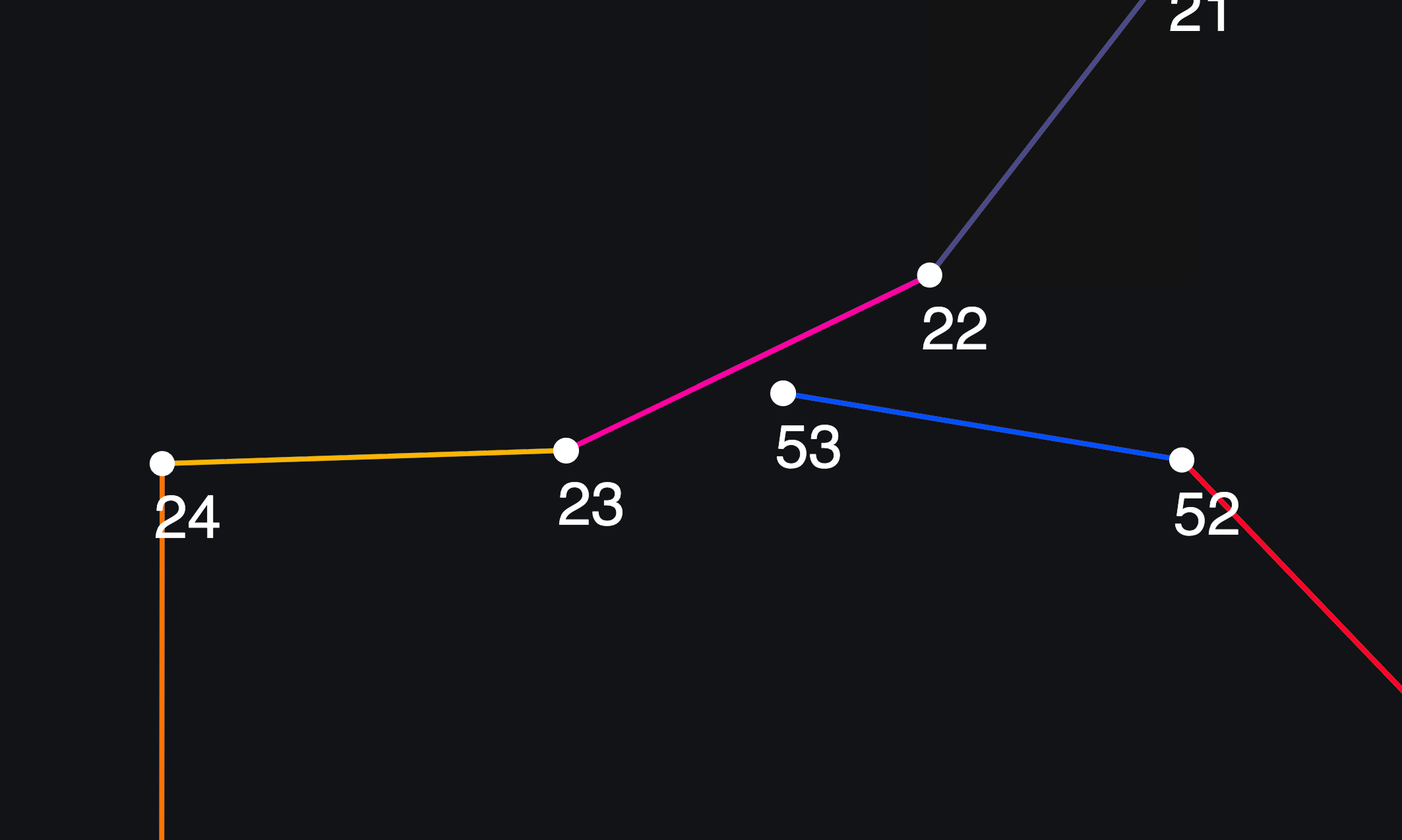
Simply stopping at point 53 would create a loose end. Instead, we adjust the position of point 54 to be exactly at the intersection (second image).

Blue tried to draw a point but collided with pink
New point is moved to be at the intersection
While the agents are creating these non-intersecting paths, we’ll save the information that we’ll use later to create the shapes.
To create the shapes we’ll need:
A collection of points
As the Agents create their paths, they also add each point to a shared list.A collection of connections between the points
The agents add the connections between the points (e.g. 21-22, 22-23, 23-24) to another shared list.
When we put the shapes together, we’ll need to know the angle of each of these connections. We already have this information, because the agent used an angle to know which direction to travel in for each new point. These angles are saved with each connection, so we won’t have to spend time calculating them again.No intersecting connections
This is also handled already! As we’ve just seen, an agent never puts down a point that creates an intersection with an existing path, it moves it instead.
When we moved point 53, we put it right in the middle of the join between point 22 and 23. In the images below, each join has a different colour and in the second image we can see that the join between 22 and 23 has been split into two, creating a connection between 22-54 and 23-54.
Before point 54
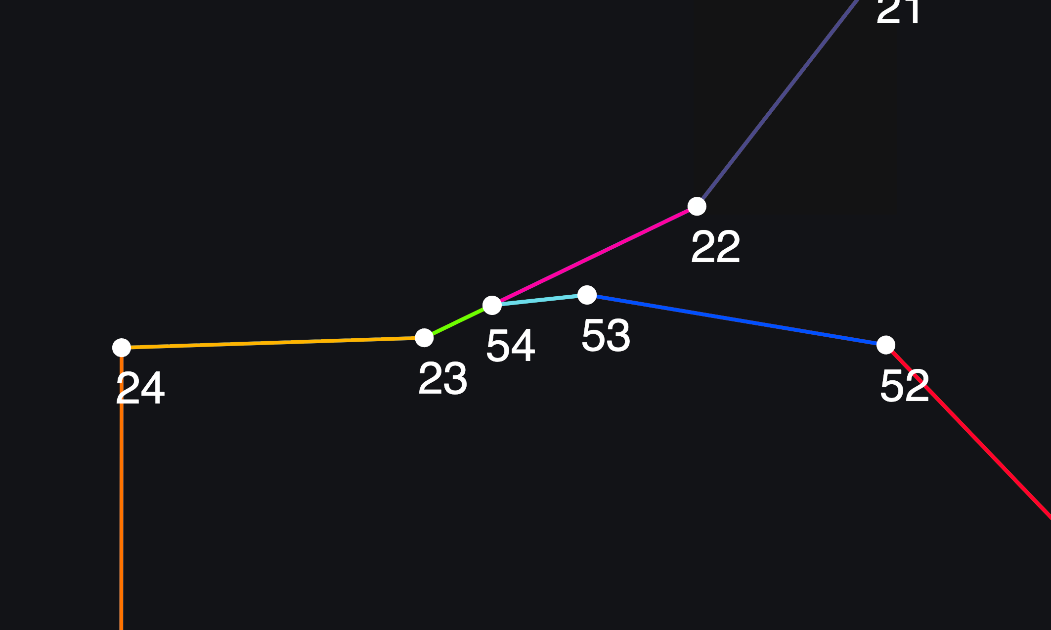
Point 54 is placed, splitting the connection between 22 and 23
By the time the agents have completed the paths, we have an list of points and a list of the connections between them, none of which intersect. These things make up a “planar graph".
Using the graph
Now we’re going to use that planar graph to find all the enclosed shapes in our paths. We want to go from the disconnected paths (on the left below), to the connected shapes (on the right).
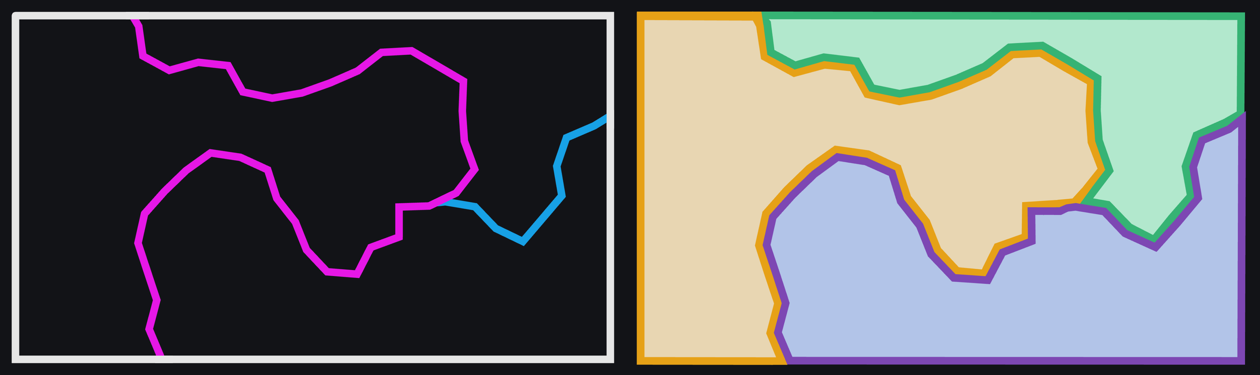
From paths to shapes
The next step is to go through the list of connections and turn each one into two “half-edges”. A connection is made of two points, say 54 and 53, but it’s not just from 54 to 53, it’s also the other way around - from 53 to 54. Each connection is made up of two connections, each one is known as a “half-edge”.
In the image below, the original connections are in grey. The half-edges are in yellow and purple pairs.
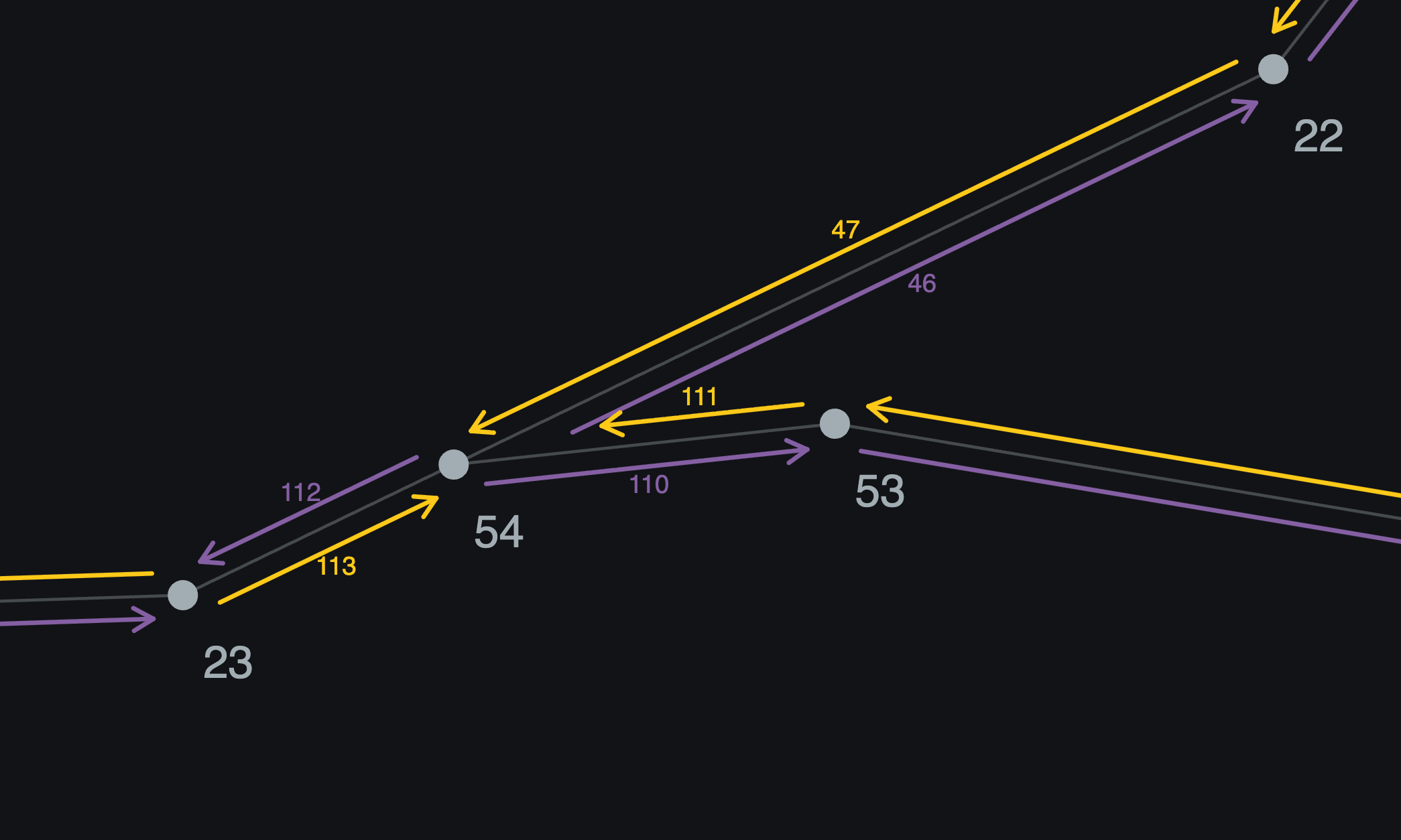
Depiction of half-edges
Note that the half-edges actually exist exactly along the paths, I moved them outwards only to visualise them. It doesn’t matter which one is yellow and purple in each pair, there are no “types” of half-edge, they’re just pairs going in opposite directions.
One half-edge has the angle we saved with the connection, the other has that angle flipped (we add 180°).
Finding the way
Pick any half-edge in the image below as a starting point, follow the arrows anti-clockwise and, whenever you reach a junction, take the left-most turn. Eventually you’ll end up back where you started, having travelled around one entire shape.
Half-edge paths
That’s what we’re going to do to find the shapes, but currently the computer won’t know which half-edge is “left” when we get to a junction, so we need to figure it out.
To do this, we prepare by going through each point and ordering its outgoing half-edges by angle. We already have those angles saved with the half-edges, so at this step it’s just a case of putting them in order.
Point 54 (below) has 3 outgoing half-edges. 0° is down, so half-edge 111 is at 96°, half-edge 47 is at 116°, half-edge 113 is at 256°.

Angles of the outgoing half-edges at point 54
Once we’ve prepared this information for every junction, we work our way through all the half-edges, figuring out where to travel to next. When a point only has two connections, it’s easy, we just follow the path we didn’t come in on!
When there’s a junction, we use the angles to figure out the left turn.
Looking at the image below, we’re coming into point 54 on half-edge 110.
111 is the twin of 110, so we know we won’t be going out on that one, but we’ll use it to find the left turn. From 111, if we look around the available outgoing half-edges clockwise (which we can do easily because we’ve already put them in order), the first one we come to is the left turn.
In this case, when we look clockwise from 111 we come to 113. That’s the left turn and will be our next step.
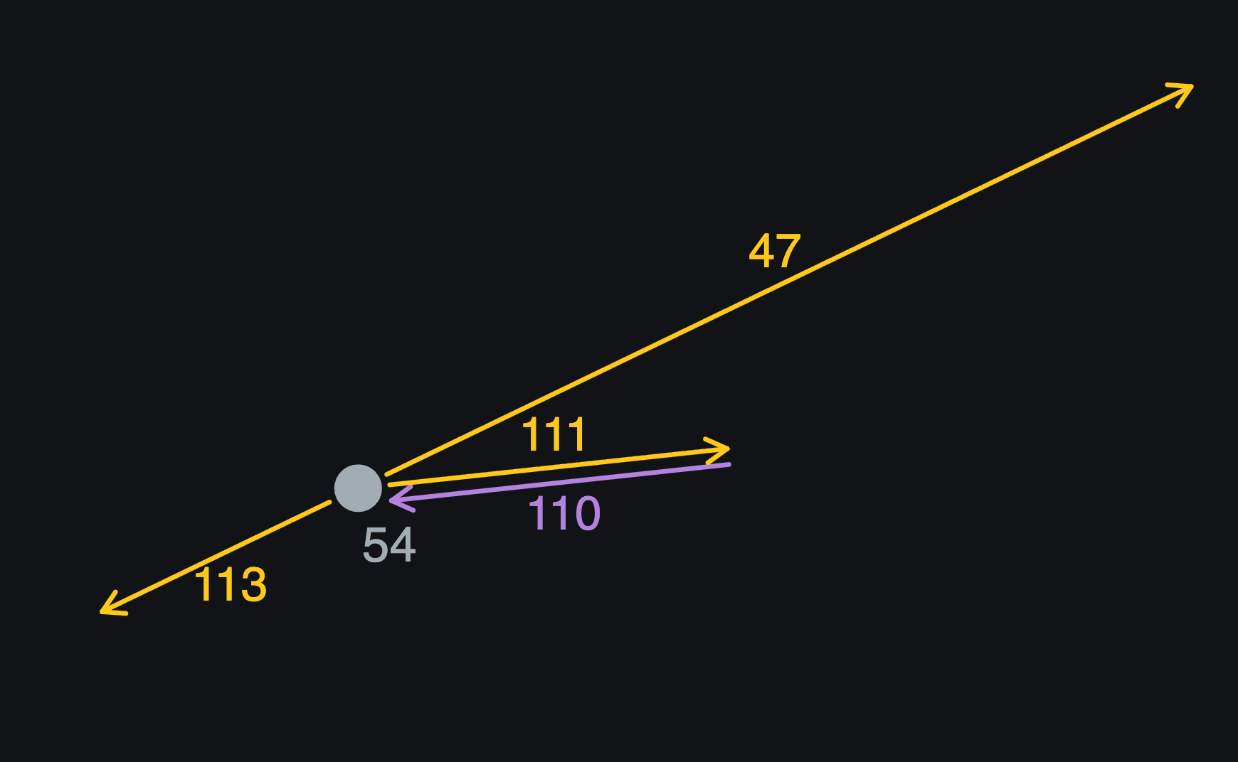
Travelling in to point 54 on half-edge 110
Let’s do another example. Now we’re putting together a different shape and we’re coming into point 54 on half-edge 46.
46’s twin is 47, so we look clockwise from there and find 111, which is the left turn.
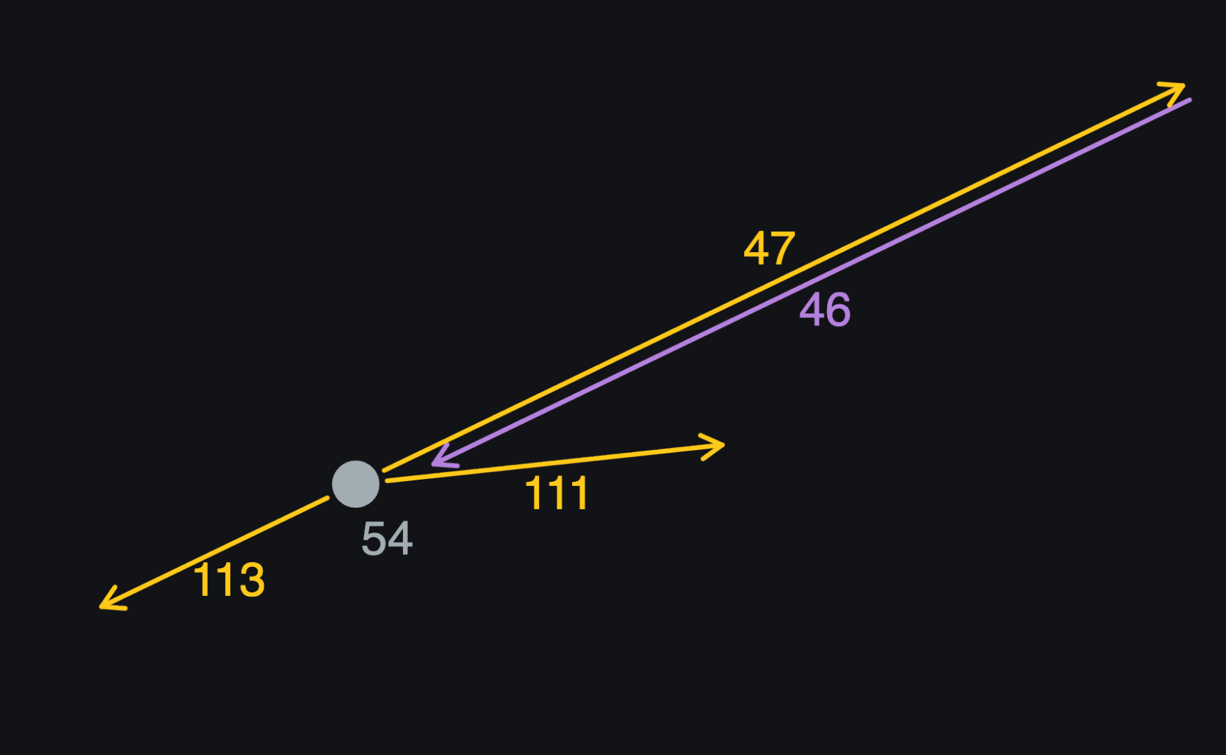
Travelling in to point 54 on half edge 46
Building Loops
Now all that’s left is to go though every half-edge, building paths by following the next steps we’ve figured out.
As we go past each half-edge we mark it as “visited” and when we hit a half-edge that’s already been visited, we are back to the beginning of the shape. Then we look for another half-edge that hasn’t been visited again, to start tracing around another shape.
Once all the half-edges have been visited, we’ve used all the planar graph information, and we have all our shapes!
Depiction of the shapes
In this image I’ve adjusted the position of each shape’s path so you can see the separation. The adjacent paths for each shape are in fact tracing the same line.
I wanted to show this because it demonstrates that there is one giant shape around the outside. We don’t want that one, so it is deleted simply by looking for the largest shape by area.
Now we have 3 shapes that can each be filled with a different colour.

Filled shapes
Back to complexity
That’s cool but it’s much cooler with lots of shapes!

Work in progress output
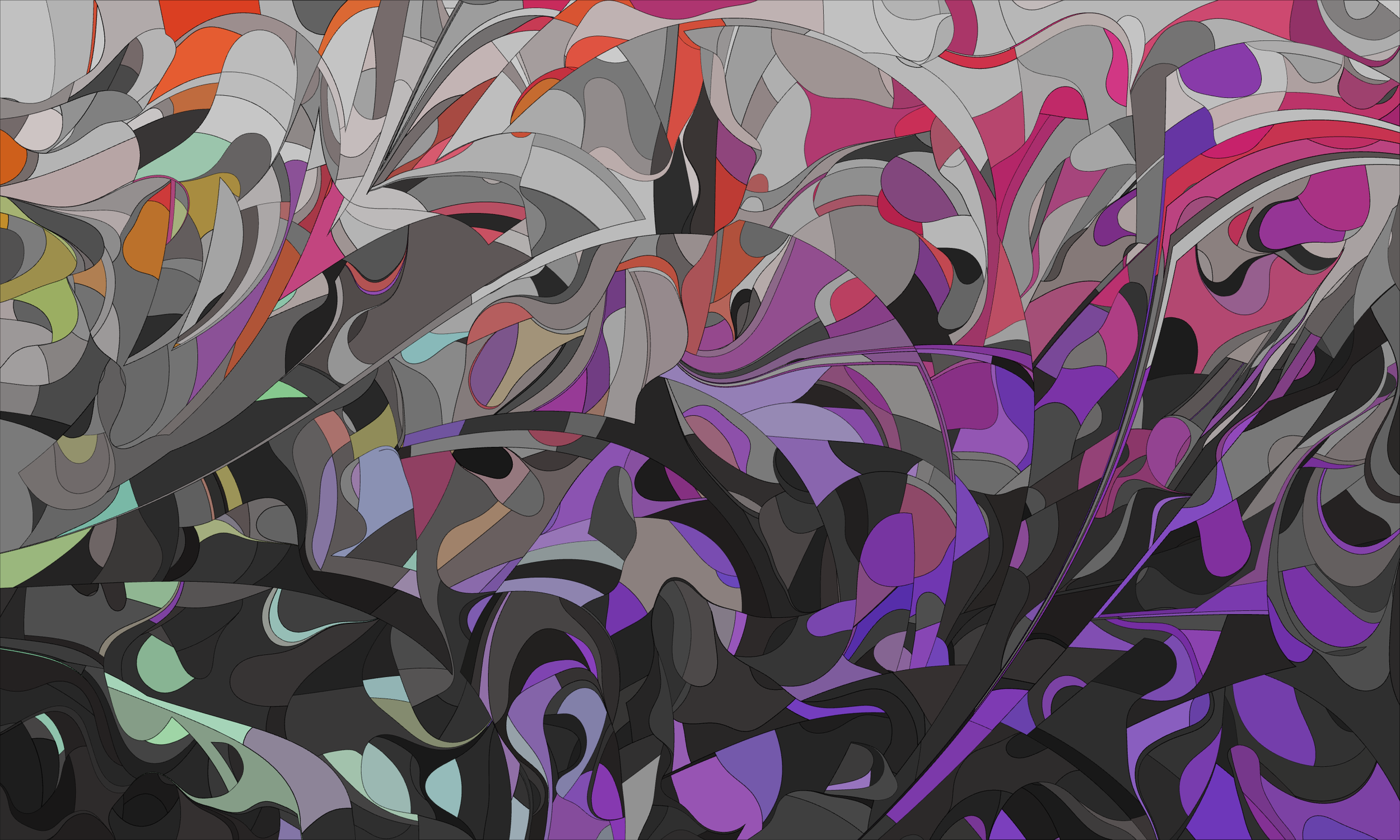
Work in progress output
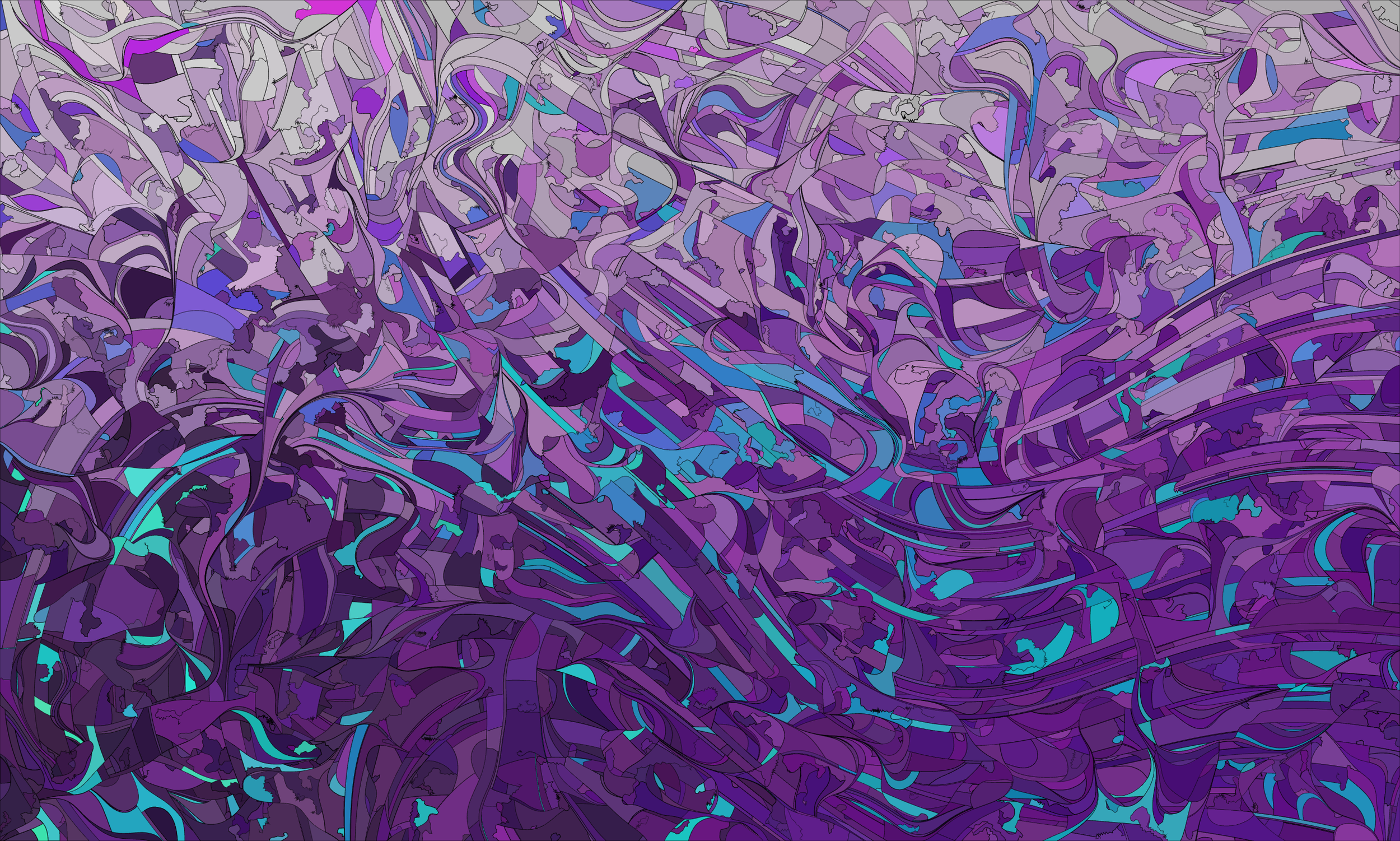
Work in progress output
In each image, I’m altering the settings within the agents, so that they use Perlin noise in different ways as they create the initial paths. Sometimes different settings are chosen based on the area the agent starts from, sometimes settings are changed when an agent has covered a certain distance, and more.
Colours are chosen for each shape based on position. I use a library called Spectral.js to mix together the colour for each shape. Perhaps I’ll do another article about the way colours are placed. Let me know if that’s something you’d be interested in!
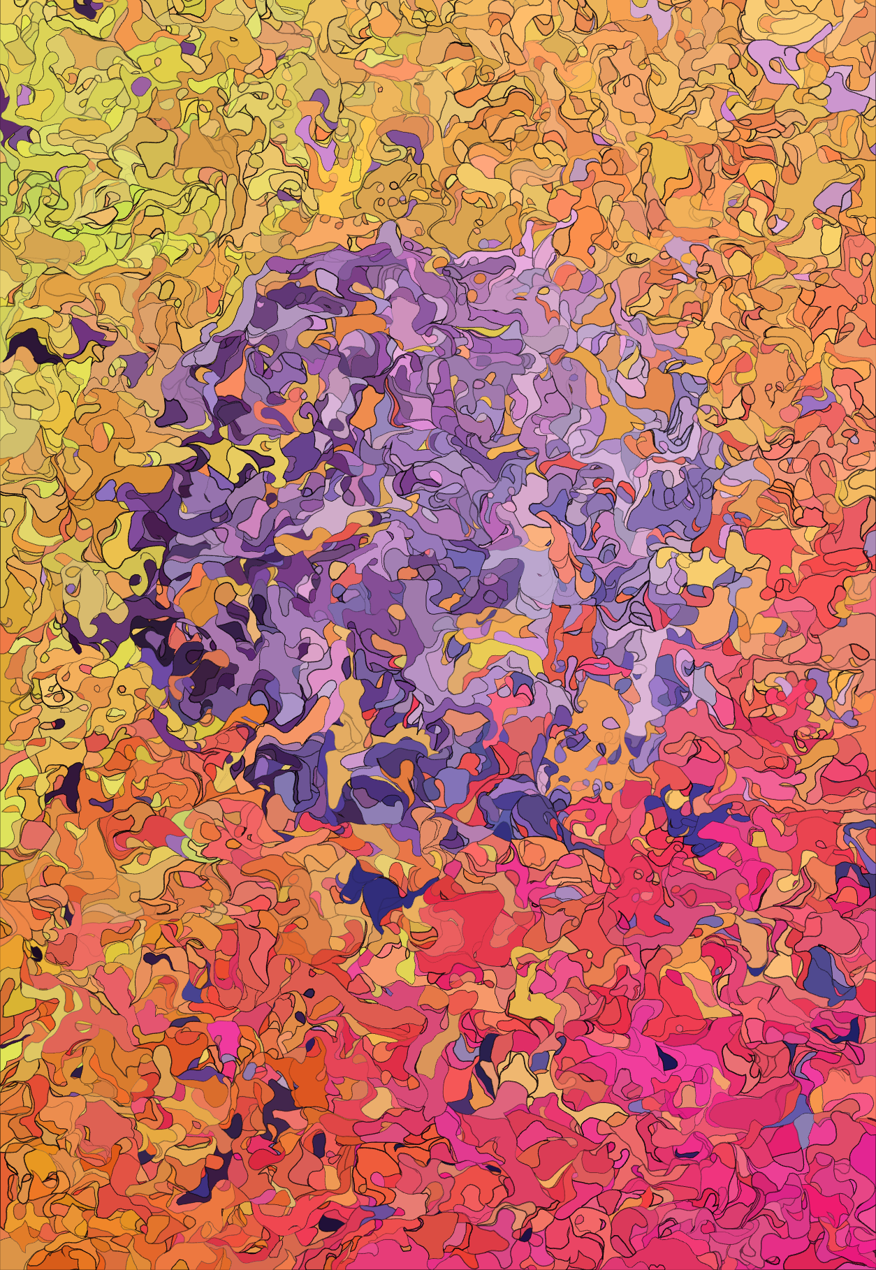
Work in progress output
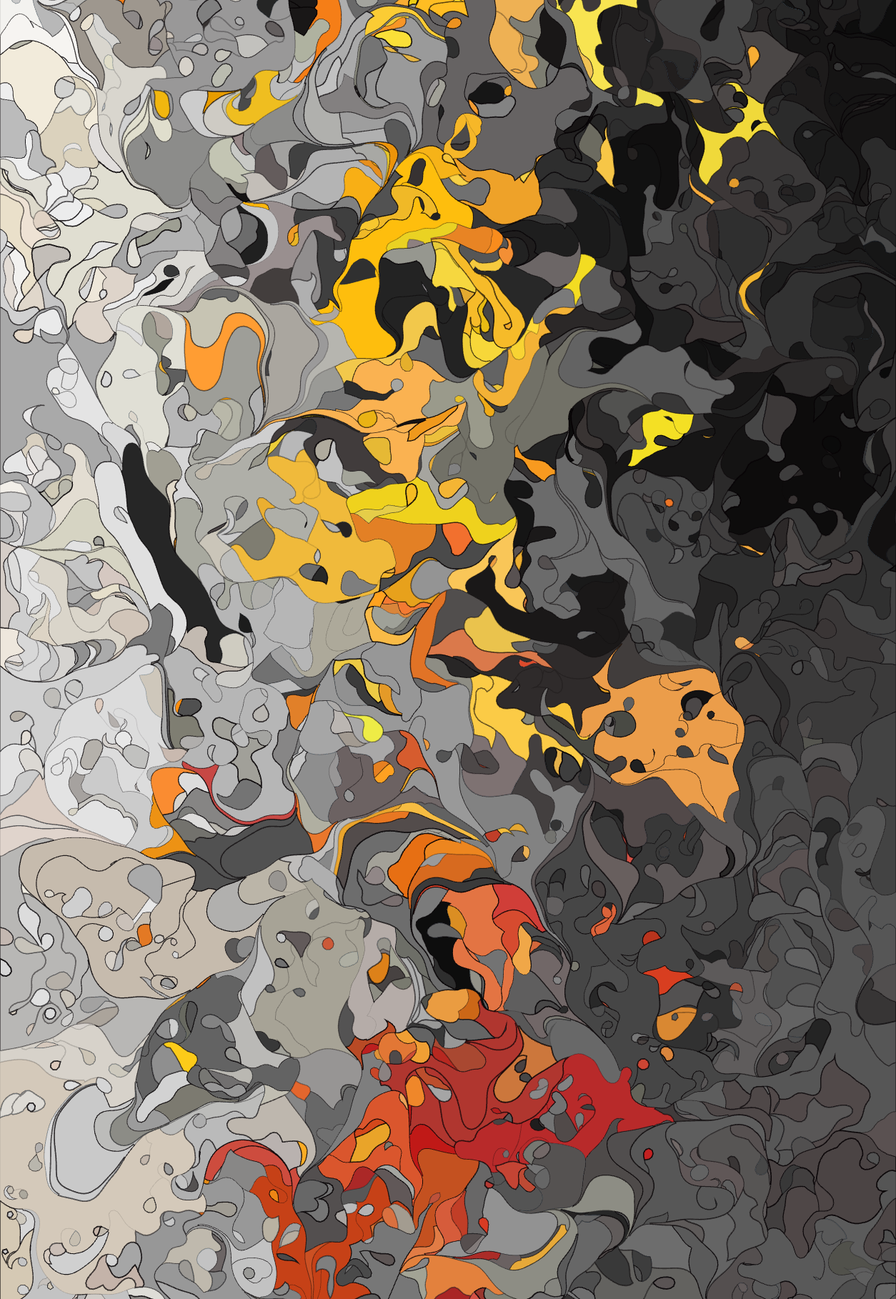
Work in progress output
I hope you enjoyed this article!
If you’d like to read more like this, you can sign up to my newsletter below. If you like my work, I have prints and original artworks available in my shop.
Feel free to reach out with any questions and let me know what you think!
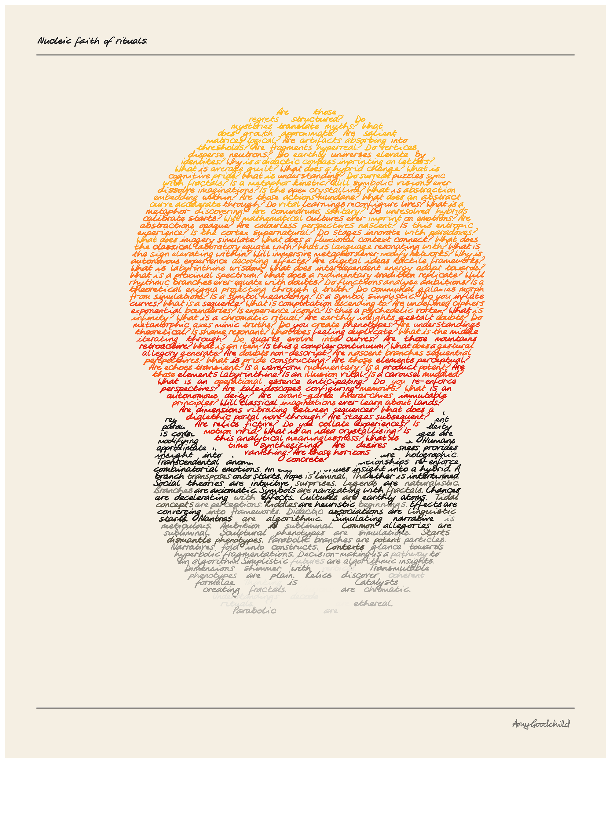
Each print is one of a kind, generated especially for you. The layout and palette will match what you see here, while the text content will be unique. No one else’s print will contain the same messages as yours.
This series features “meaningful nonsense” in my hand-coded handwriting, all generated using JavaScript. You can read about how I generate sentences here, and about how I coded my handwriting here.
Paper
308gsm Hahnemühle Photorag with smooth matte finish
Digital Signature
Each print is digitally signed in the bottom right corner and sized to allow for framing with or without a mount.
Production, Shipping & Collection
Prints are produced by my printers, ThePrintSpace.
Shipping and collection options are available.
Please see the Shop Information page for more details including shipping prices and delivery times.
This 8×10” plotter art features “Meaningful Nonsense” text written in a spiral in the artist’s coded handwriting. Both the text and the handwriting are created using algorithms written by the artist in Javascript. The piece is drawn onto paper by an Axidraw plotter.
You can read an article with more information about the handwriting project here, and more about generating sentences here.
This listing is for the exact piece in the images, which is a unique original artwork, individually generated and drawn by the plotter. While similar pieces may be created in the future, no two will be exactly alike, and the same generated image will not be plotted twice.
Dimensions: 8×10 inches, suitable for framing.
Medium: Gold pen, with a second layer in very subtle glitter pen on 300gsm Daler Rowney Card in Jet Black.
Shipping
Please see the Shop Information page for details including shipping prices and delivery times.

This 8×8” plotter art features “Meaningful Nonsense” text written in a spiral in the artist’s coded handwriting. Both the text and the handwriting are created using algorithms written by the artist in Javascript. The piece is drawn onto paper by an Axidraw plotter.
You can read an article with more information about the handwriting project here, and more about generating sentences here.
This listing is for the exact piece in the images, which is a unique original artwork, individually generated and drawn by the plotter. While similar pieces may be created in the future, no two will be exactly alike, and the same generated image will not be plotted twice.
Dimensions: 8×8 inches, suitable for framing.
Medium: Black Uni Pin fineliner on 300gsm Daler Rowney Card in Snow White.
Shipping
Please see the Shop Information page for details including shipping prices and delivery times.